Empirical Modeling of the Geomagnetic Field

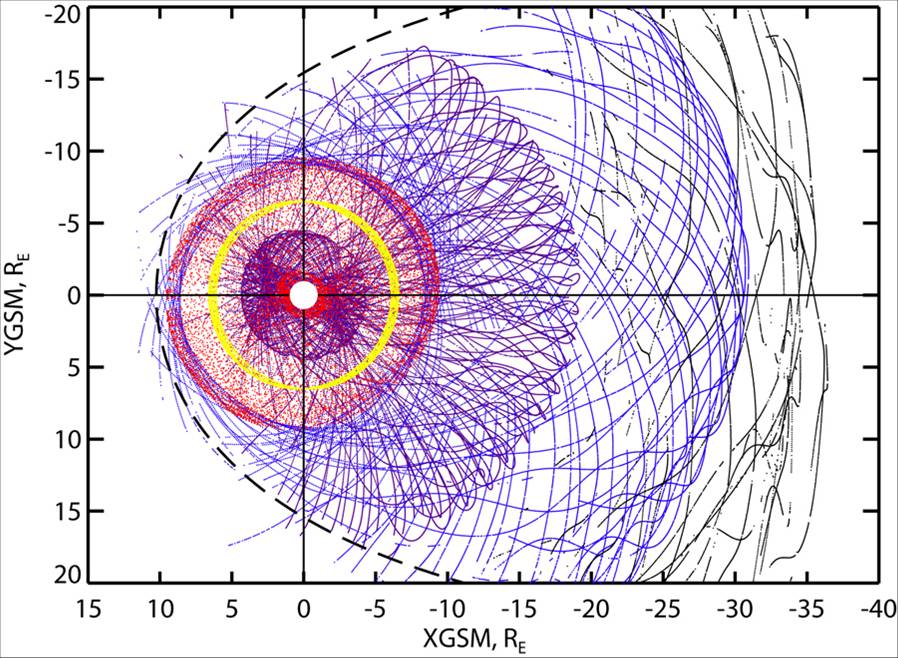
In contrast to many popular renditions, the actual magnetosphere is mostly invisible. Only at high latitudes and relatively close to Earth, particle precipitation along magnetic field lines forms impressive "light festivals" known as auroral borealis and astralis (northern and southerns auroras, respectively). Some other regions of the magnetosphere can also be made "visible" due to the charge exchange between ions and neutral atoms that are also present in the magnetosphere close to Earth. The resulting flux of neutral atoms can be seen using special ENA detectors on several missions, such as IMAGE and TWINS. At the same time, a vast quantity of data is being accumulated due to in-situ measurements of the magnetospheric magnetic field. These data represent an extremely attractive resource for empirical modeling and vizualization of the magnetosphere, especially during magnetic storms. Spatial distribution of the data records in a subset of data of Polar, GOES-12, CLUSTER, Geotail, and IMP 8 satellites is shown in the left panel of Figure 1. These data, combined with new data-processing techniques make it possible to reconstruct the structure and dynamics of the storm-time magnetosphere with an unprecedented resolution (Figure 2, right panel). This approach complements the first-principle modeling of the magnetosphere using global MHD simulations and special "ring current" models some of which are now available through the Community Coordinated Modeling Center (CCMC). The present website gives a brief overview of the current empirical models of the geomagnetic field and underlying current systems with the emphasis on a detailed description of the high-resolution model TS07D (Tsyganenko and Sitnov, 2007; Sitnov, Tsyganenko, Ukhorskiy, and Brandt, 2008). Figure 1. Distribution of magnetic field data measurements in the magnetosphere (left) and results of the empirical reconstruction of the magnetospheric current systems based on such data (right). Left panel shows projections on the equatorial plane of measurement locations for subsets of data taken from Polar (red), GOES-12 (yellow), CLUSTER (magenta), Geotail (blue), and IMP 8 (black) satellites (Tsyganenko et al., Eos Trans. AGU, 89(53), Fall Meet. Suppl., SM14A-02). Animation in the right panel shows results of the dynamical reconstruction of the April 2001 magnetic storm using the new high-resolution empirical geomagnetic field model (Tsyganenko and Sitnov, 2007) and the advanced data-mining techniques (Sitnov, Tsyganenko, Ukhorskiy, and Brandt, 2008). Distribution of the equatorial current density vectors and their directions are shown by the color coding and arrows, respectively. The corresponding phase of the storm is marked by the red diamond in the plot of the Sym-H index (inset).

In classical empirical geomagnetic field models the magnetic field is presented as a sum of the internal (core) field (IGRF) and a few modules representing the principal magnetospheric current systems: 1) Chapman-Ferraro current confining the dipole field inside the magnetopause; 2) the tail current closed via the magnetopause; 3) symmetric ring current; 4) partial ring current; 5) Birkeland currents, connecting the ionosphere with the solar wind (Region 1 currents) or with the partial ring current (Region 2). The geometry of each module is fixed and based in particular on some physical principles. For example, the Chapman-Ferraro current system must cancel the component of the dipole field normal to the magnetopause, while the tail current system must be located near the equatorial plane, taking into account hinging, twisting, and warping effects of the magnetotail current sheet. Note that each magnetospheric current system is independently shielded (has its own subsystem of Chapman-Ferraro-type currents at the magnetopause). Individual contributions of the modules to the total magnetic field are determined by the corresponding amplitude coefficients and are found by fitting the model to available measurements of the geomagnetic field. The amplitude coefficients are either binned by the activity level (e.g., Kp index) or are some pre-defined functions of the solar wind plasma parameters (density and velocity) and the interplanetary magnetic field.

The above approach was motivated by the sparseness of in-situ data in the magnetosphere and in the solar wind. The dramatic increase of the amount of data that has become possible in the last decade due to single-probe GOES, Geotail and Polar missions as well as multi-probe Cluster and Themis constellations, allowed us to develop an advanced, qualitatively new approach to the empirical modeling. The resulting new model differs from the classical models in two important aspects. First, the magnetic field of all the equatorial currents (tail and ring systems and their shielding subsystems) is described now by a regular expansion into a series of basis functions that allows for any distribution of currents in the equatorial sheet with a finite thickness. The spatial resolution of such an expansion is determined by the number of terms in the expansion and can be increased to any desired level, commensurate with the data density. Second, instead of the past model parametrizations based on either binning data by the activity level (T89 model) or global fitting using the whole database of solar wind, IMF and magnetospheric data (T96, T01, and TS05 models), the new model employs a dynamical data mining approach based on the concept of the nearest neighbors (NN). In this approach, at every moment of time the spatial distribution of the magnetospheric currents is found using an individual subset of the whole database. It includes both the actual data obtained for the given state of the magnetosphere and data from other time intervals (e.g., similar phases of other storms) that neighbor the given state in the space of the global parameters, solar wind electric field, pressure-corrected Sym-H index, and its time derivative. Two other important parameters, the dipole tilt angle and the solar wind dynamic pressure are built in the main spatial structure of the model and they can be excluded from the above data mining procedure. With the presently used database including more than 10⁶ points and NN~8·10³ points used for the reconstruction of each magnetic field "snapshot", the model is highly nonlinear. In particular, even for relatively strong storms with minimum Sym-H ~ -100nT, the difference between the actual Sym-H averaged in time over few hours and its value averaged over NNs does not exceed ~5%.

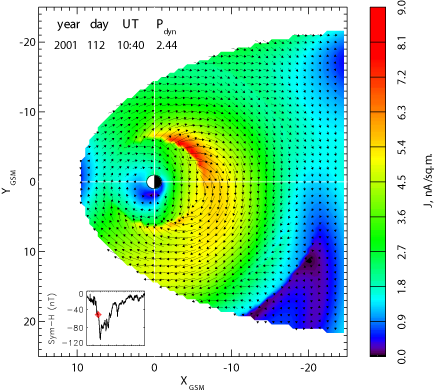
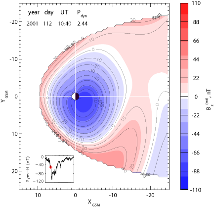
Figures 2 and 3 below, together with the animation in the right panel of Figure 1 show possible outputs of the new model. Figure 2 shows the distribution of the equatorial current density (left) and the external magnetic field component normal to the equatorial plane. For simplicity, in plotting these parameters the tilt angle changes in the model output were not taken into account, although they were taken into account in the fitting procedure.

<

Figure 2. Distribution of the equatorial current density (left) and the external magnetic field component normal to the equatorial plane (right) in the main phase of the April 2001 magnetic storm (from Sitnov, Tsyganenko, Ukhorskiy, and Brandt, 2008).

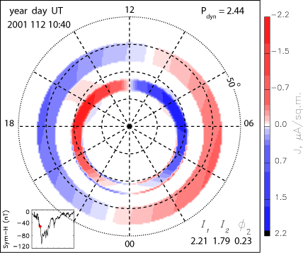
Tilt angle effects are shown in the left panel of Figure 3 in a picture of magnetic field lines and the dawn-dusk component of the current density in the meridional plane. The right panel shows the corresponding distribution of Birkeland currents at the ionospheric level, where the parameters I₁, I₂, and f₂ in the right bottom corner indicate the amplitudes of the Region 1 and Region 2 currents in MAs and the westward rotation angle of the Region 2 system.

Figure 3. Magnetic field lines, the color-coded dawn-dusk component of the current density (left) and the distribution of Birkeland currents at the ionospheric level in the main phase of the April 2001 magnetic storm (Sitnov, Tsyganenko, Ukhorskiy, and Brandt, 2008).

The source code of the TS07D model can be found HERE. Its interface is similar in structure to previous models, such as TS05 (see classical empirical geomagnetic field models). However, the use of the code has two important distinctions. First, it requires a set of AUXILIARY FILES 'tail*.par' that contain the amplitudes of the shielding coefficients for all basis functions of the equatorial current system (presently their number is 45). Second, the input of the code requires, along with the GSM coordinates of the point, where the magnetic field is calculated, and the time, also the value of the dynamical pressure PDYN and the set of dynamical code coefficients, which is found using the data mining (NN) procedure and a fitting code, and which is unique for the given moment in time (note, that the time value is also used to calculate the tilt angle). At present, the state parameters are provided in the following LIST OF PROCESSED STORMS with 1 hour interval (the highest temporal resolution of the present model is 5 min). The performance of the code is not limited to storms, although the NN search involves a few-hour averaging in time and thus reflects largely storm time scales. We plan to populate the list of available events as a part of the specific research projects. The RUN ON REQUEST tool, combining the aforementioned data mining and fitting procedures and covering the period 1995-2005 (in-sample modeling regime, corresponding to the extension of the present model database), is now available.

As is seen from the above, TS07D is complementary both to the available first-principle models and to the existing empirical geomagnetic field models. The price for high resolution in space and high flexibility in time variations is quite high for the present model. The need to re-calculate the model coefficients at every new moment in time makes it similar in performance to the present first-principle MHD and the ring current models. Note, that although the latter models are presently limited in the global description of the magnetosphere, potentially they should provide the most comprehensive information on its structure and dynamics, including both the magnetic field and other key parameters, such as the electric field and plasma moments. At the same time, the information on the global structure of the magnetic field and global current distribution provided by the present model may help in benchmarking and coupling of the aforementioned first-principle models as well as in the data assimilation.

Some of the past empirical models may be more appropriate, compared to to the present model, when, for instance, the magnetic field update frequency is critical or the role of the specific solar wind parameters, plasma density, velocity of the magnetic field clock angle needs to be clarified (see classical empirical geomagnetic field models). Moreover, even the semi-empirical magnetic field models using very limited data for their fitting may be of use and importance. The examples are event-oriented and hybrid-input algorithms (Kubyshkina, Sergeev, and Pulkkinen, 1999), which are used for modeling of substorms and sawtooth events, as well as the paraboloid model (Alexeev et al., 1999; 2001), which turned out to be surprisingly efficient in the draft models of other planetary magnetospheres. Another example is the description of the innermost eastward current, which exists at distances closer than ~ 3R_E due to the positive radial gradient of the plasma pressure. It is not reproduced by the present version of the model, mostly because the currently used database contains relatively little data at radial distances less than 4R_E. At the same time, the innermost eastward current can be described using other data from ISEE, AMPTE/CCE and Polar satellites and different empirical approaches (Le, Russell, and Takahashi, 2004). Besides, a relatively rigid structure of the present model in the decription of the low altitude Birkeland currents is complemented by the detailed empirical picture of those currents inferred from the Iridium constellation and the DMSP data.